Top 15 Excel functions for accountants: take your Excel skills to the next level!

Excel has been the go-to spreadsheet tool for accountants since its launch in the mid-1980s. Decades later, and despite the advent of AI-driven automation, many accountants still rely on Excel to record and analyze financial data.

Yet despite its somewhat basic appearance, there’s more to Excel than meets the eye. By mastering its basic formulas and functions, you can save time, reduce errors, and increase efficiency. In this article, we’ll explore 15 of the most important Excel functions — and how to use them in accounting. 

15 Excel functions for accountants to master

Here are 15 top formulas to transform how you use Excel. 

• SUM
• AVERAGE
• VLOOKUP
• IF
• SUMIF
• COUNTIF
• ROUND
• PMT
• NPV
• SLN
• FV
• LARGE
• SMALL
• SEQUENCE
• SORT

But before we get started, it’s worth noting that while Excel is still an effective tool for analyzing financial information, running an efficient and profitable accounting practice requires more than just spreadsheets.

Instead of relying on outdated tools, forward-thinking firms use practice management software such as TaxDome, where you can centralize all your client data, communications, and processes in one place. The result is automated processes, enhanced accuracy and efficiency, and a superior client experience. 

1. SUM

The SUM function is perhaps the most well-known and well-used Excel formula. As the name suggests, it’s used to add up a range of values, providing you with a total, or sum. 

Here’s what the formula looks like: 

=SUM(insert cell range)

To add a range, simply drag and hold your cursor over the cells you want to add up, like in the example below. As you can see, the start and end cells of the range are separated by a colon.

For more complex additions, you can add multiple ranges and individual cells by separating them with commas. The same goes for other formulas in this list. Here’s an example:

How accountants can use it

You can use the SUM function to quickly find the total value of different columns of financial data. For example, you can use SUM to calculate total expenses, revenues, account balances, or payroll totals. 

2. AVERAGE 

Excel’s AVERAGE function allows you to calculate the average of a range of values with ease. It’s one of the most basic yet crucial formulas to know. 

Here’s what the syntax looks like: 

=AVERAGE(insert cell range)

How accountants can use it

There are countless ways you can use the AVERAGE function as an accountant, but here are just a few examples:

• Calculating the average sales for a quarter
• Determining average monthly expenses over the course of a year
• Finding the average salary of employees in a particular department

3. VLOOKUP

VLOOKUP is a very useful function that enables you to take a piece of information in one list (a name, value, date, etc.), look up that data in another list, and then return another piece of data related to that information. 

In the screenshot below, for example, we have a list of names on the left and an empty job titles column. On the right, we have another list, containing names, employer numbers, and job titles. As you can see, the job title column in this list is filled. 

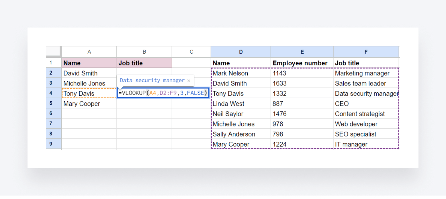
Say we want to add Tony Davis’ job title to the list on the left by referencing the list on the right. We would start by writing this:

=VLOOKUP

Then, in parentheses, we’d add:

• The cell containing the lookup value, i.e. Tony Davis’ name (A4)
• The range in the second list where the value we want to find (Tony Davis) is located (D2:F9)
• The column number within that range containing the value we want to return (3)

Additionally, you can add FALSE if you want an exact match or TRUE if you want an approximate match. So, the final syntax looks like this:

=VLOOKUP(A4, D2:F9, 3, FALSE)

How accountants can use it

Again, there are limitless possibilities for using VLOOKUP, but here are a few examples to illustrate its functionality:

• Retrieve a client’s phone number using their client ID
• Find the due date of an invoice using the invoice number
• Identify the cost of an item using its product number

4. IF

IF is another essential Excel function to learn. It enables you to make a logical comparison between one piece of data and another. If the first piece of data meets certain criteria, you can set the function to return a specific term. If it doesn’t meet the criteria, you can set the function to return a different term. 

Let’s look at an example. Below, we have a list of employees, their performance ratings, and a performance benchmark. If their performance exceeds the benchmark, the employee is eligible for a bonus. The IF function can help speed up this process.

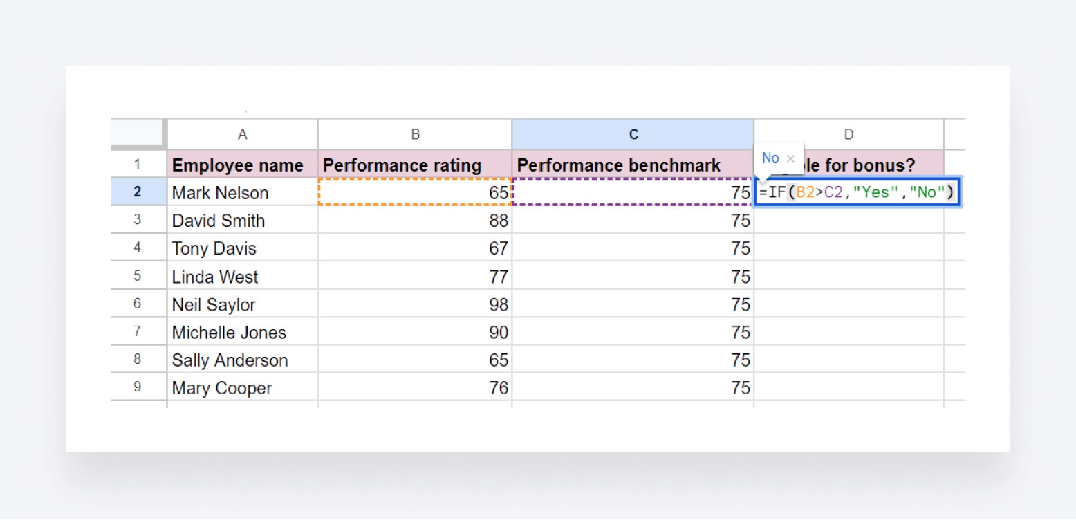
If we want to find out if Mark Nelson is eligible for a bonus, you would write the function like this: 

=IF(B2>C2, “yes”, “No”)

In other words, if the value in cell B2 is greater than the value in cell C2, return “Yes”. If it isn’t, return “No”. 

You can then extrapolate that logic across all rows, like this:

How accountants can use it

You can use the IF function in any scenario where you want to apply simple logic to a value. Here are just a few examples:

• Determining if an invoice is overdue or not
• Checking if expenses are over or under budget
• Verifying whether a customer qualifies for a discount based on their purchase amount

5. SUMIF

A combination of the SUM and IF functions, SUMIF adds together the values in cells that meet a specified condition or criteria. 

In the example below, we want to find the total of all purchases requiring approval. The approval threshold is $1000.

To calculate this, we write: 

=SUMIF(A2:A9, “>999”)

In other words, we are asking the function to calculate the total of all values in the range A2 to A9 that are larger than 999. 

How accountants can use it

SUMIF is a very flexible function with many use cases. Here are just a few examples of how you can use it in accounting:

• Finding the total amount of expenses for a specific business department or team
• Calculating the total sales amounts that are greater than a specified value
• Adding up all travel expenses that exceed a certain amount

6. COUNTIF

Similar to the SUMIF function, COUNTIF counts the number of cells that meet a certain criterion. In the example below, we are using COUNTIF to calculate how many sales a certain salesperson — in this case, Sarah — has made.

To do this, we write: 

=COUNTIF(B2:B10, “Sarah”)

In other words, how many times does the term “Sarah” appear in the range from cell B2 to B10? Of course, this can work for numbers, dates, or any other kind of data as well.

How accountants can use it

Here are just some of the ways accountants can use COUNTIF to speed up data analysis:

• Counting the number of overdue invoices
• Counting the number of transactions over a certain amount
• Counting the number of sales relating to a certain product or service line

7. ROUND

Sometimes, for the sake of clarity, you might want to round numbers up or down to the nearest decimal point. With the ROUND function, you can do this with ease. See the example below:

If we want to round up the sales amounts to the nearest dollar, we write the formula like this:

=ROUND(A2,0) 

In this example, the zero indicates no decimal points. If you want to round the amount to one decimal place, you would write it like this:

=ROUND(A2,1) 

How accountants can use it

In addition to rounding sales figures, you can use the ROUND function to:

• Round numbers with a large number of decimal places to two decimal places, to represent the value in dollars and cents
• Round commission amounts to the nearest dollar

8. PMT

One of the more finance-focused functions on this list, PMT enables you to calculate the amount of money you will need to repay for a loan based on three inputs: 

• A constant interest rate 
• The number of repayment periods
• The loan amount, or principal

Here’s an example.

To calculate the yearly repayment amount, we would write:

=PMT(B1, B2, B3)

You can also calculate the monthly repayment like this:

=PMT(B1/12, B2*12, B3)

Note how we are dividing the interest amount by 12 to account for 12 monthly payments, and then multiplying the number of years by 12 for the same reason. See the example below:

How accountants can use it

Accountants can use the PMT function to calculate repayments for any kind of loan, from financial loans to leased equipment, vehicles, or property. You can change the loan repayment period as well, calculating amounts for monthly, quarterly, or annual payments, for example.

9. NPV

NPV is a powerful function that enables you to calculate the net present value of an investment based on future cash flows and a discount rate. The discount rate represents the fact that money available today is worth more than the same amount in the future because it can be invested and earn returns in the meantime. 

Essentially, understanding NPV helps accountants and business leaders determine whether an investment is viable or not, making it a crucial tool for financial modeling and budgeting.

Let’s look at the example below in Excel. 

As you can see, we are looking at making a $500k investment this year. Over the next five years, we expect the investment to yield the returns you can see in column C. The discount rate we are using is 10%. 

To calculate the net present value, we would write: 

=NPV(B10, C3:C7)+C2

Note how the range includes just the years when there is positive cash flow, and after the parenthesis, we add the amount that we initially invested. The NPV comes out at just over $16k, so this is indeed a viable investment!

How accountants can use it

The NPV function can be used to help stakeholders understand the potential value of an investment. You can apply it to everything from small, low-risk investments such as IT infrastructure or software development to large, high-risk investments such as acquiring a company or building a new plant.

10. SLN

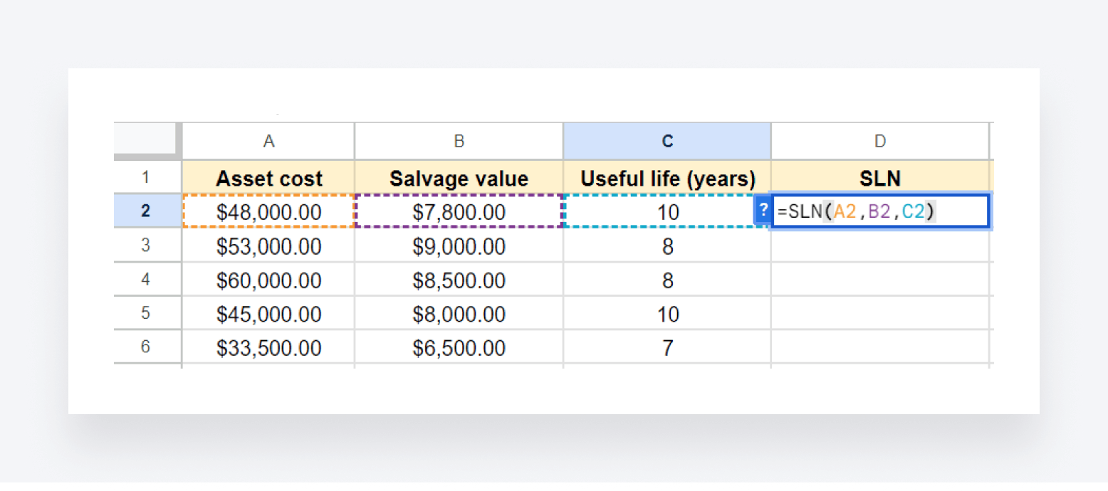
Another useful function for accountants, SLN calculates the straight-line depreciation of an asset over one period of time. To calculate SLN, you need to know: 

• The initial cost of the asset
• The value of the asset at the end of its useful life (also known as the salvage value)
• The number of years or months over which the asset will depreciate (also known as the useful life of the asset)

In Excel, the syntax looks like this:

=SLN(cost, salvage, life)

For the first asset in the example below, that would look like this:

=SLN(A2,B2,C2)

Just a reminder that in Excel, you can copy the function across all rows by dragging and dropping the blue dot in the bottom left corner of a cell. See below:

How accountants can use it

You can use the SLN function to calculate the straight-line depreciation of any asset, including office equipment, vehicles, manufacturing machinery, and more. This helps you understand how the value of your assets decreases over time, helping you to plan and analyze financial performance more accurately.

 11. FV

Another financial function, FV enables you to calculate the future value of an investment based on a constant interest rate. To do this, you need to know three following pieces of information: 

• The interest rate per period
• The total number of periods
• The amount invested per period

In addition, there are two optional pieces of information you can add: 

• Whether the investments are made at the beginning or the end of the period
• The initial account value

Let’s take a look at an example in Excel:

As you can see, we’ve written the function like this: 

=FV(B2/12, B3*12, -B4, -B1)

In other words, we’ve taken the rate of return and divided it by 12 to reflect the fact we’re making monthly investments. We’ve then added the number of years, which we’ve multiplied by 12 for the same reason. We then minus the monthly investment and do the same for the initial account value. 

Note: you can also specify when during the period the payment will be made. If you make your investments at the end of the period, you can add a zero (this is the default option). If you make your investments at the beginning of the period, add the number one.

How accountants can use it

Accountants can use the FV formula to understand the future value of an investment, assuming the rate of return stays the same. In practice, they could use it to:

• Forecast expected future returns for clients interested in investing
• Calculate the future value of cash savings in a savings account

12. LARGE

The LARGE function enables you to identify the largest number in a range — or the second largest, or the third largest, and so on, depending on what you add to the formula. It’s a more flexible version of the MAX function, which only allows you to find the largest value in a range. 

In the example below, we want to find the biggest sale from a range of different values. 

To do this, we write:

=LARGE(B2:B7, 1)

In other words, we are asking the function to look in the cell range from B2 to B7 for the largest value. To find the second largest value, simply change the ‘1’ in the formula to ‘2’, and so on for the second, third, or fourth-largest — you get the picture. 

How accountants can use it

The LARGE function is a relatively simple tool, but it can save accountants a lot of time when identifying values of a particular size relative to others within a range. For example, you could use it to find the highest revenue in a list of earnings, the second-biggest supplier payment, the third-highest expense, and so on.

13. SMALL

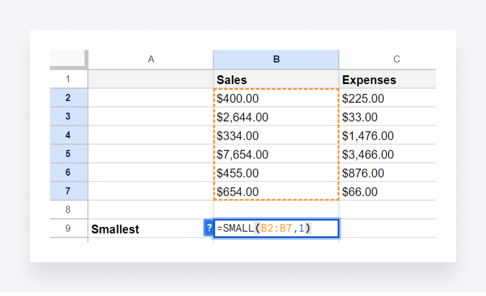
The opposite of LARGE, the SMALL function helps you find the smallest (or second-smallest, or third-smallest, etc.) value in a range. 

The syntax works the same as the LARGE function, with the inputs being the range of cells you want to search and then a number representing the relative order of smallness you are looking for, with one for the smallest, two for the second-smallest, and so on. See below:

How accountants can use it

You can use SMALL to identify the smallest revenue, expense, or invoice. You could also use it to identify the worst-performing accounting period. 

14. SEQUENCE

The SEQUENCE function is a handy tool that enables you to generate a sequence of numbers based on specific inputs, including:

• The number of rows
• The number of columns
• The starting value
• The step for each subsequent value in the sequence

Say we want to quickly create a list of ten invoice numbers, starting with 1001 and increasing by 1 each time. We’d write:

=SEQUENCE(10, 1, 1001, 1) 

In other words, we’re asking the formala to create a sequence of numbers that’s 10 rows long, 1 column wide, starting with 1001, and increasing by 1 each time. Here’s what we get: 

Now, let’s say that we need to create a sequence of dates, starting with the first date of the year and with each subsequent date being seven days later. Let’s also say that we want this list to be 40 dates long and presented on a table comprising 10 rows and 4 columns. We would write:

=SEQUENCE(10, 4, DATE(2024, 1, 1), 7)

Again, 10 here represents the number of rows, 4 represents the number of columns, DATE represents the date, and 7 represents the sequence logic.

Here’s what we’d get:

How accountants can use it

There are all sorts of ways accountants can use the SEQUENCE function, from numbering transactions and invoices to identifying periodic deadlines for reporting, client communication, or internal reviews.

15. SORT

The SORT function organizes a list of values, names, dates, or any other information into a logical order. In the example below, we organized a random list of sales figures into ascending order by adding the cell range (A2:A10) to the function: 

=SORT(A2:A10)

If you want to organize the list of sales figures along with their associated salespeople, you can do it like this:

=SORT(A2:B10,2,1)

In this case, we highlight the entire range (A2:B10), then add the column we want to sort (2). The final “1” indicates that we want the array organized in ascending order. For descending order, we’d have to write “-1”. 

Conclusion

Decades after its launch, Excel remains a useful tool for accountants looking to analyze financial data. But to truly unlock its potential, you need to master its many functions. The 15 formulas we’ve covered in this article are a great place to start, enabling you to sort, calculate, and manipulate data quickly and accurately. 

That said, spreadsheets have their limitations. To run a truly efficient and profitable accounting practice, you need to move beyond outdated tools and practices and use technology that promotes accuracy, efficiency, and quality across all of your workflows.

With TaxDome, you have a centralized system for managing all your data, tools, and processes. From automating workflows to managing clients, staff, and projects, it can be the operating system for your practice.